Tutorial¶

[1]:

# NBVAL_IGNORE_OUTPUT
%load_ext watermark
import numpy as np
import qutip
import matplotlib
import matplotlib.pylab as plt
import weylchamber
from weylchamber.visualize import WeylChamber
%watermark -v --iversions

Python implementation: CPython
Python version       : 3.9.7
IPython version      : 8.1.1

numpy      : 1.21.2
qutip      : 4.6.3
matplotlib : 3.5.1
weylchamber: 0.3.2+dev

\(\newcommand{Re}[0]{\operatorname{Re}} \newcommand{Im}[0]{\operatorname{Im}} \newcommand{dd}[0]{\,\text{d}} \newcommand{abs}[0]{\operatorname{abs}}\)

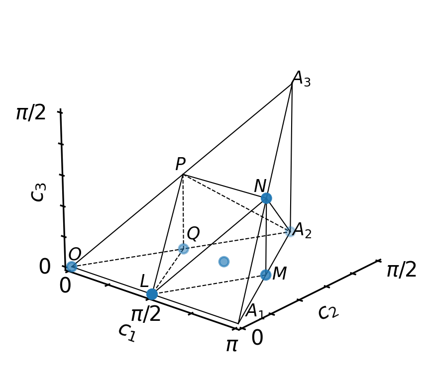
Every two-qubit gate is associated with a point in the “Weyl-chamber” that may be visualized in three dimensions as the following polyhedron:

[2]:

WeylChamber().plot()

Note: if you run this interactively, and switch to an interactive matplotlib backend, e.g.

%matplotlib tk

you will be able to rotate the 3D plot to get a better intuition.

Consider the following common two-qubit gates:

[3]:

IDENTITY = qutip.identity([2,2])
IDENTITY

[3]:

Quantum object: dims = [[2, 2], [2, 2]], shape = (4, 4), type = oper, isherm = True\begin{equation*}\left(\begin{array}{*{11}c}1.0 & 0.0 & 0.0 & 0.0\\0.0 & 1.0 & 0.0 & 0.0\\0.0 & 0.0 & 1.0 & 0.0\\0.0 & 0.0 & 0.0 & 1.0\\\end{array}\right)\end{equation*}

[4]:

CNOT = qutip.qip.operations.cnot()
CNOT

[4]:

Quantum object: dims = [[2, 2], [2, 2]], shape = (4, 4), type = oper, isherm = True\begin{equation*}\left(\begin{array}{*{11}c}1.0 & 0.0 & 0.0 & 0.0\\0.0 & 1.0 & 0.0 & 0.0\\0.0 & 0.0 & 0.0 & 1.0\\0.0 & 0.0 & 1.0 & 0.0\\\end{array}\right)\end{equation*}

[5]:

CPHASE = qutip.qip.operations.cphase(np.pi)
CPHASE

[5]:

Quantum object: dims = [[2, 2], [2, 2]], shape = (4, 4), type = oper, isherm = True\begin{equation*}\left(\begin{array}{*{11}c}1.0 & 0.0 & 0.0 & 0.0\\0.0 & 1.0 & 0.0 & 0.0\\0.0 & 0.0 & 1.0 & 0.0\\0.0 & 0.0 & 0.0 & -1.0\\\end{array}\right)\end{equation*}

[6]:

BGATE = qutip.qip.operations.berkeley()
BGATE

[6]:

Quantum object: dims = [[2, 2], [2, 2]], shape = (4, 4), type = oper, isherm = False\begin{equation*}\left(\begin{array}{*{11}c}0.924 & 0.0 & 0.0 & 0.383j\\0.0 & 0.383 & 0.924j & 0.0\\0.0 & 0.924j & 0.383 & 0.0\\0.383j & 0.0 & 0.0 & 0.924\\\end{array}\right)\end{equation*}

[7]:

iSWAP = qutip.qip.operations.iswap()
iSWAP

[7]:

Quantum object: dims = [[2, 2], [2, 2]], shape = (4, 4), type = oper, isherm = False\begin{equation*}\left(\begin{array}{*{11}c}1.0 & 0.0 & 0.0 & 0.0\\0.0 & 0.0 & 1.0j & 0.0\\0.0 & 1.0j & 0.0 & 0.0\\0.0 & 0.0 & 0.0 & 1.0\\\end{array}\right)\end{equation*}

[8]:

sqrtISWAP = qutip.qip.operations.sqrtiswap()
sqrtISWAP

[8]:

Quantum object: dims = [[2, 2], [2, 2]], shape = (4, 4), type = oper, isherm = False\begin{equation*}\left(\begin{array}{*{11}c}1.0 & 0.0 & 0.0 & 0.0\\0.0 & 0.707 & 0.707j & 0.0\\0.0 & 0.707j & 0.707 & 0.0\\0.0 & 0.0 & 0.0 & 1.0\\\end{array}\right)\end{equation*}

[9]:

sqrtSWAP = qutip.qip.operations.sqrtswap()
sqrtSWAP

[9]:

Quantum object: dims = [[2, 2], [2, 2]], shape = (4, 4), type = oper, isherm = False\begin{equation*}\left(\begin{array}{*{11}c}1.0 & 0.0 & 0.0 & 0.0\\0.0 & (0.500+0.500j) & (0.500-0.500j) & 0.0\\0.0 & (0.500-0.500j) & (0.500+0.500j) & 0.0\\0.0 & 0.0 & 0.0 & 1.0\\\end{array}\right)\end{equation*}

[10]:

MGATE = weylchamber.canonical_gate(3/4, 1/4, 0)
MGATE

[10]:

Quantum object: dims = [[2, 2], [2, 2]], shape = (4, 4), type = oper, isherm = False\begin{equation*}\left(\begin{array}{*{11}c}0.707 & 0.0 & 0.0 & 0.707j\\0.0 & 0.0 & 1.0j & 0.0\\0.0 & 1.0j & 0.0 & 0.0\\0.707j & 0.0 & 0.0 & 0.707\\\end{array}\right)\end{equation*}

All of these gates are situatated at special points in the Weyl chamber. We can print their Weyl chamber coordinates and add a point in the graphical representation

[11]:

w = WeylChamber();
list_of_gates = [
    ('Identity', IDENTITY),
    ('CNOT', CNOT), ('CPHASE', CPHASE), ('BGATE', BGATE),
    ('iSWAP', iSWAP), ('sqrtISWAP', sqrtISWAP),
    ('sqrtSWAP', sqrtSWAP), ('MGATE', MGATE)]
print("Weyl Chamber Coordinates")
print("----------------------------------")
for (name, gate) in list_of_gates:
    c1, c2, c3 = weylchamber.c1c2c3(gate)
    print("%10s: \t%.2fπ %.2fπ %.2fπ" % (name, c1, c2, c3))
    w.add_point(c1, c2, c3)
w.plot()

Weyl Chamber Coordinates
----------------------------------
  Identity:     0.00π 0.00π 0.00π
      CNOT:     0.50π 0.00π 0.00π
    CPHASE:     0.50π 0.00π 0.00π
     BGATE:     0.50π 0.25π 0.00π
     iSWAP:     0.50π 0.50π 0.00π
 sqrtISWAP:     0.25π 0.25π 0.00π
  sqrtSWAP:     0.75π 0.25π 0.25π
     MGATE:     0.75π 0.25π 0.00π

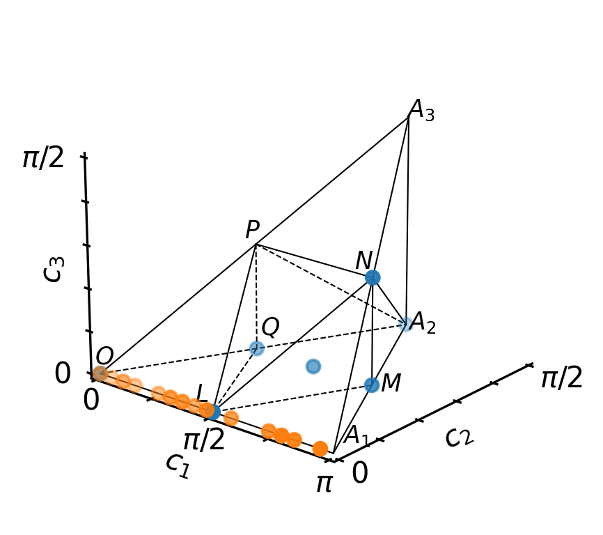
The gates locally equivalent to the controlled-phase gates are on an the axis 0 - A1 in the Weyl chamber:

[12]:

w.scatter(*zip(*[
    weylchamber.c1c2c3(qutip.qip.operations.cphase(phase))
    for phase in np.linspace(0, 2*np.pi, 20)]))

[13]:

w.plot()

The Weyl chamber coordinates \((c_1, c_2, c_3)\) are closely associated with the local invariants \((g_1, g_2, g_3)\)

[14]:

print("Local Invariants")
print("----------------------------------")
for (name, gate) in list_of_gates:
    g1, g2, g3 = weylchamber.g1g2g3(gate)
    print("%10s: \t%5.2f %5.2f %5.2f" % (name, g1, g2, g3))

Local Invariants
----------------------------------
  Identity:      1.00  0.00  3.00
      CNOT:      0.00  0.00  1.00
    CPHASE:      0.00  0.00  1.00
     BGATE:      0.00 -0.00  0.00
     iSWAP:      0.00  0.00 -1.00
 sqrtISWAP:      0.25  0.00  1.00
  sqrtSWAP:      0.00 -0.25  0.00
     MGATE:      0.25  0.00  1.00

This shows that the MGATE and \(\sqrt{\text{iSWAP}}\) are actually locally equivalent, despite being different Weyl chamber coordinates (M and Q, respectively)